Modeling of spatially varying phenomena based on landscape similarity to stratification units. If each stratification unit across geographic space represents a distinct landscape configuration (in terms of multiple landscape factors and/or factor scales), and if each landscape configuration influences a phenomenon in a distinct way, then the spatial variability of that phenomenon can be assessed across a landscape by relating each geographic location to each distinct landscape configuration. Therefore, the more similar a geographic location is to the landscape configuration represented by a given stratification unit, then also the more similar the response of a phenomenon will be at that location to the typical response for conditions within the given stratification unit. Both continuous and categorical response variables are supported. For categorical responses, each category must be identified by an integer value.
Usage
engine(
  res.type = "cont",
  ls.rast,
  n.win = 3,
  su.repobs,
  tiles,
  parallel = FALSE,
  outdir = ".",
  tile.rm = TRUE,
  extension = ".tif",
  verbose = FALSE,
  ...
)
Arguments
- res.type
Character. Type of response to model. Options are "cont" for continuous, and "cat" for categorical response. Default: "cont"
- ls.rast
SpatRaster, as in
rast. Multi-layer SpatRaster representing landscape similarities to stratification units. Only similarities for units with a representative observation are allowed. Character prefix in the file name of similarities is allowed.- n.win
Integer. Positive number indicating how many winning stratification units should be considered. See Details. Default: 3
- su.repobs
Data frame. The first column of this data frame must contain only the numeric code for the stratification units (without prefix). Each additional column must contain the value of the representative response observation for each stratification unit. Multiple response variables are allowed (one per column). Note that all response variables in the data frame must share the same type (res.type). See example on issues related to non-explicit column names.
- tiles
SpatVector, as in
vect. Spatial vector of polygon geometry with the boundaries of the area of interest. This vector can be subdivided in regions (i.e., tiles) to balance memory allocation and processing speed (see Details). If this vector is tiled, then its attribute table must only contain an ID column with a unique identifier for each tile (1,2,...,n). Additionally, This vector must have the same coordinate reference system as ls.rast.- parallel
Boolean. Perform parallel processing? A parallel backend needs to be registered beforehand with
registerDoParallel. Moreover, a tiled spatial vector should be supplied for tiles. Default: FALSE- outdir
Character. String specifying the path for the output raster tiles/layer(s) of modeled response(s). Default: "."
- tile.rm
Boolean. Should the tiles of modeled response(s) be removed from disk after the tile merging process? Default: TRUE
- extension
Character. String specifying the extension for the output raster layer(s) of modeled response(s). Default: ".tif"
- verbose
Boolean. Show warning messages in the console? Default: FALSE
- ...
Additional arguments as for
writeRaster.
Details
The predictive modeling process is cell-wise, which means that it operates on a cell-by-cell basis. For a given cell occurring in the geographic space supported by a raster layer, the predictive modeling engine first identifies the n stratification units to which the given cell is most similar (i.e., 'winning stratification units'). The engine is able to identify the winning stratification units thanks to the user-provided set of landscape similarity layers ls.rast. Subsequently, the response value from the representative observation for each winning stratification unit is identified. In the case of a continuous response, a weighted average of representative response values is performed. For each representative response value, the weight is proportional to the corresponding stratification unit's landscape similarity value in the given cell. The result of the weighted average is assigned as the response value in the given cell. In the case of a categorical response, the modal value from the representative response values of the n winning stratification units is assigned to the given cell.
Note that the name for each raster layer in ls.rast should match the
numeric code of the corresponding stratification unit, which is obtained from
the column of numeric codes in su.repobs. Nevertheless, raster layer
names in ls.rast with a character prefix in the numeric code and/or
file extension should work fine (e.g., "su_1101.tif" instead of "1101"). If
the landscape similarity layers in ls.rast were created with
similarity, then raster layer names will not have any prefix
nor extension as part of the numeric code.
When dealing with large geographic spaces, high raster resolutions (i.e., small cell sizes), or both, a considerable amount of memory is required to perform the modeling process. To reduce memory usage, the predictive modeling engine performs tile-based processing of landscape similarity layers and writes results directly on disk. Tile-based processing increases the computational time, thus parallelization is allowed by setting up a parallel backend. If parallelization is enabled, then care must be taken with the size of the tiles since larger sizes will have a greater impact on memory usage. Consequently, the parallel, tile-based processing will be less useful.
Examples
require(terra)
p <- system.file("exdat", package = "rassta")
# Multi-layer SpatRaster of landscape similarities
fls <- list.files(path = p, pattern = "su_", full.names = TRUE)
ls <- terra::rast(fls)
# Numeric code and representative response value for stratification units
fro <-list.files(path = p, pattern = "repobs.csv", full.names = TRUE)
ro <- read.csv(fro)
# Extract only those stratification units with representative value
ls <- ls[[as.character(ro$SU)]]
# SpatVector with processing tiles
fti <- list.files(path = p, pattern = "tiles.shp", full.names = TRUE)
ti <- terra::vect(fti)
# Directory for temporary files
o <- tempdir()
# Perform predictive modeling of continuous response
r <- engine(res.type = "cont", ls.rast = ls, n.win = 2, su.repobs = ro,
tiles = ti, outdir = o, overwrite = TRUE
)
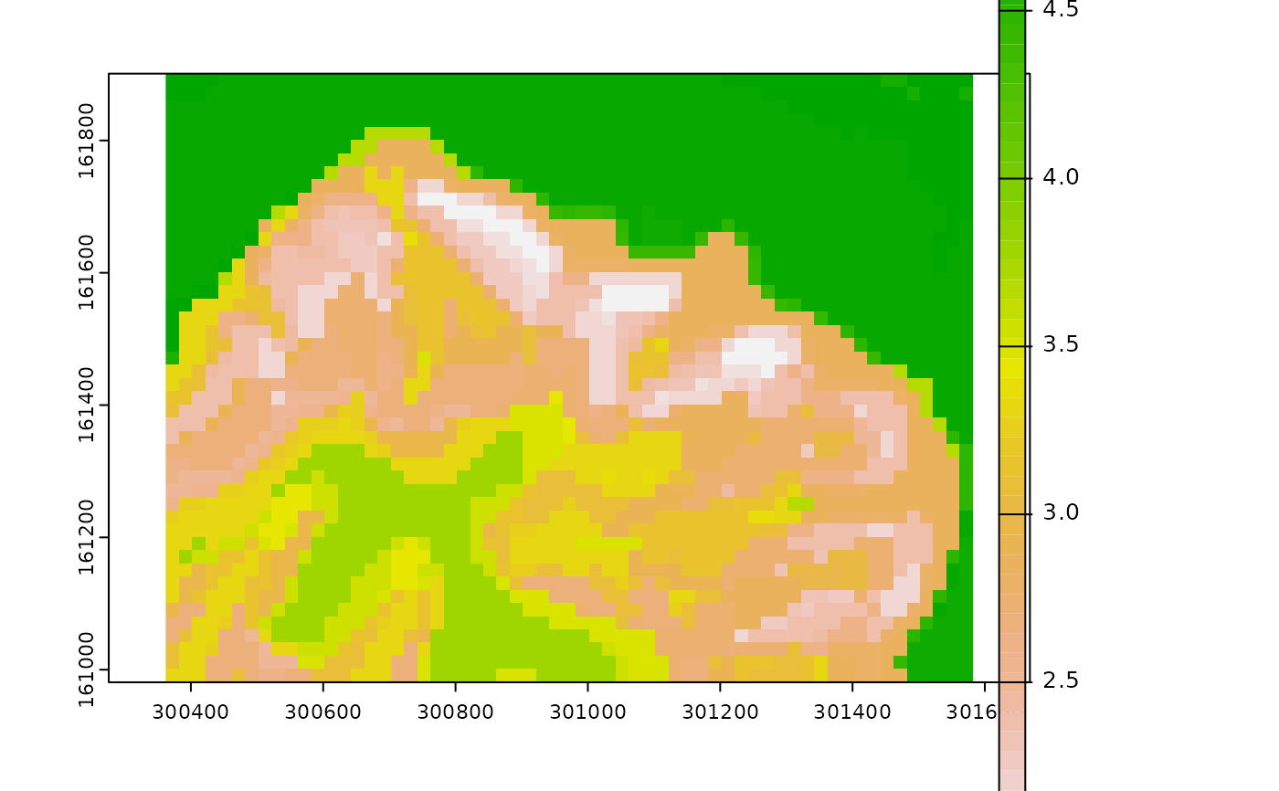
# Plot modeled response
if(interactive()){plot(r)}
 # Clean temporary files
file.remove(list.files(path = o, pattern = "soc.tif", full.names = TRUE))
#> [1] TRUE
#
#-------
# A note on non-explicit response's names (obtained from su.repobs):
## This will result in incorrectly modeled response values
x <- c("SOM", "SOM_30cm", "SOM_45cm") # SOM = soil organic matter
grep(x[1], x) # Non explicit
#> [1] 1 2 3
grep(x[2], x) # Explicit
#> [1] 2
grep(x[3], x) # Explicit
#> [1] 3
## This will result in correct values
x <- c("SOM_15cm", "SOM_30cm", "SOM_45cm")
grep(x[1], x) # Explicit
#> [1] 1
grep(x[2], x) # Explicit
#> [1] 2
grep(x[3], x) # Explicit
#> [1] 3
# Clean temporary files
file.remove(list.files(path = o, pattern = "soc.tif", full.names = TRUE))
#> [1] TRUE
#
#-------
# A note on non-explicit response's names (obtained from su.repobs):
## This will result in incorrectly modeled response values
x <- c("SOM", "SOM_30cm", "SOM_45cm") # SOM = soil organic matter
grep(x[1], x) # Non explicit
#> [1] 1 2 3
grep(x[2], x) # Explicit
#> [1] 2
grep(x[3], x) # Explicit
#> [1] 3
## This will result in correct values
x <- c("SOM_15cm", "SOM_30cm", "SOM_45cm")
grep(x[1], x) # Explicit
#> [1] 1
grep(x[2], x) # Explicit
#> [1] 2
grep(x[3], x) # Explicit
#> [1] 3