Predict Distribution Functions Across Geographic Space

Predicts constrained, univariate distribution functions across the geographic space supported by raster layers. For a given continuous variable used to create a classification unit, this function first calculates a user-defined distribution function for that variable using only observations selected from within the classification unit. In this way, the distribution function is univariate and constrained. Subsequently, a locally-estimated scatterplot smoothing (LOESS) or a generalized additive model (GAM) is fitted. This model is fitted using the variable’s observations as explanatory values and the values from the distribution function as the response values. Finally, the fitted model is predicted on the complete geographic space supported by the raster layer of the given variable. This process is iterated for all of the continuous variables and classification units. Each resulting layer can be thought of as a landscape correspondence measurement between an XY location in geographic space and the landscape configuration represented by a given classification unit in terms of a specific variable. The following distribution functions are currently supported: the probability density function (PDF), the empirical cumulative density function (ECDF), and the inverse of the empirical cumulative density function (iECDF). Please refer to Details for more information about how each distribution function is calculated. Also, see details on parallel processing.

Usage

predict_functions(
  cuvar.rast,
  cu.ind,
  cu,
  vars,
  dif,
  hist.type = "regular",
  hist.pen = "default",
  grid.mult = 1,
  kern = "normal",
  quant.sep = 0.01,
  method = "loess",
  span = 0.6,
  k = 20,
  discrete = TRUE,
  to.disk = FALSE,
  outdir = ".",
  prefix = "",
  extension = ".tif",
  overwrite = FALSE,
  verbose = FALSE,
  ...
)

Arguments

cuvar.rast: SpatRaster, as in rast. Multi-layer SpatRaster containing n continuous raster layers (i.e., variables) and one raster layer of classification units with integer cell values (i.e., Numeric identifiers).
cu.ind: Integer. Position (index) of the raster layer of classification units in cuvar.rast.
cu: Integer. Vector of integer values that correspond to the numeric identifiers of the units in the raster layer of classification units.
vars: Character. Vector of strings containing the names of the n continuous variables in cuvar.rast. These names have to be sequentially repeated according to the number of classification units (See Examples).
dif: Character. Vector of strings containing the distribution function to calculate for each continuous variable within each classification unit. The function will match the position of the name of the distribution function with that of the name of the continuous variable in vars.
hist.type: Character. Type of histogram to calculate. Options are "regular", "irregular" (unequally-sized bins, very slow), and "combined" (the one with greater penalized likelihood is returned). See histogram. Default: "regular"
hist.pen: Character. Penalty to apply when calculating the histogram (see histogram). Default: "default"
grid.mult: Numeric. Multiplying factor to increase/decrease the size of the "optimal" grid size for the Kernel Density Estimate (KDE). Default: 1
kern: Character. Type of kernel to use for the KDE. Default: "normal"
quant.sep: Numeric. Spacing between quantiles for the calculation of the ECDF and iECDF. Quantiles are in the range of 0-1 thus spacing must be a decimal. Default: 0.01
method: Character. Model to fit. Current options are "loess" for locally-estimated scatterplot smoothing (see loess), and "gam" for generalized additive model with support for large datasets (see bam). Default: "loess"
span: Numeric. If method = "loess", degree of smoothing for LOESS fitting. Default: 0.6
k: Numeric. If method = "gam", Number of knots for the cubic regression splines. Default: 20
discrete: Boolean. If method = "gam", discretize variables for storage and efficiency reasons? Can reduce processing time significantly. Default: TRUE
to.disk: Boolean. Write the output raster layers of predicted distribution function to disk? See details an example about parallel processing. Default: FALSE
outdir: Character. If to.disk = TRUE, string specifying the path for the output raster layers of predicted distribution function. Default: "."
prefix: Character. If to.disk = TRUE, string specifying a prefix for the file names of the output raster layers of predicted distribution function. Default: ""
extension: Character. If to.disk = TRUE, string specifying the extension for the output raster layers of predicted distribution function. Default: ".tif"
overwrite: Boolean. If to.disk = TRUE, should raster layers in disk and with same name as the output raster layer(s) of predicted distribution function be overwritten? Default: FALSE
verbose: Boolean. Show warning messages in the console? Default: FALSE
...: If to.disk = TRUE, additional arguments as for writeRaster.

Value

Single-layer or multi-layer SpatRaster with the predicted distribution function for each variable and for each classification unit.

Details

To calculate the PDF, this function uses the binned KDE for observations drawn from the breaks of a regular/irregular histogram. The "optimal" number of bins for the histogram is defined by calling the function histogram (Mildenberger et al., 2019) with the user-defined penalty hist.pen. Subsequently, the optimal number of bins is treated as equivalent to the "optimal" grid size for the binned KDE. The grid size can be adjusted by specifying the multiplying factor grid.mult. Lastly, the "optimal" bandwidth for the binned KDE is calculated by applying the direct plugin method of Sheather and Jones (1991). For the calculation of optimal bandwidth and for the binned KDE, the package KernSmooth is called. To calculate both the ECDF and the iECDF, this function calls the ecdf function on equally-spaced quantiles. The spacing between quantiles can be manually adjusted via quant.sep. In the case of iECDF, the ECDF is inverted by applying the formula: iECDF = ((x - max(ECDF)) * -1) + min(ECDF); where x corresponds to each value of the ECDF.

The "cu", "vars", and "dif" parameters of this function are configured such that the output table from select_functions can be used directly as input. (see Examples).

When writing output raster layer to disk, multiple distribution functions can be predicted in parallel if a parallel backend is registered beforehand with registerDoParallel. Keep in mind that the function may require a large amount of memory when using a parallel backend with large raster layers (i.e., high resolution and/or large spatial coverage).

Some issues have been reported when manually creating cluster objects using the parallel package. To overcome this issue, a cluster object can be registered directly through registerDoParallel without passing it first through makeCluster. See examples.

References

T. Mildenberger, Y. Rozenholc, and D. Zasada. histogram: Construction of Regular and Irregular Histograms with Different Options for Automatic Choice of Bins, 2019. https://CRAN.R-project.org/package=histogram

S. Sheather and M. Jones. A reliable data-based bandwidth selection method for kernel density estimation. Journal of the Royal Statistical Society. Series B. Methodological, 53:683–690, 1991.

Examples

require(terra)
p <- system.file("exdat", package = "rassta")
# Multi-layer SpatRaster of topographic variables
## 3 continuous variables
ftva <- list.files(path = p, pattern = "^height|^slope|^wetness",
                   full.names = TRUE
                  )
tva <- terra::rast(ftva)
# Single-layer SpatRaster of topographic classification units
## Five classification units
ftcu <- list.files(path = p, pattern = "topography.tif", full.names = TRUE)
tcu <- terra::rast(ftcu)
# Add the classification units to the SpatRaster of topographic variables
tcuvars <- c(tcu, tva)
# Data frame with source for "cu", "vars", and "dif"
ftdif <- list.files(path = p, pattern = "topodif.csv", full.names = TRUE)
tdif <- read.csv(ftdif)
# Check structure of source data frame
head(tdif)
#>   Class.Unit Variable Dist.Func
#> 1          1   height      ECDF
#> 2          1    slope       PDF
#> 3          1  wetness       PDF
#> 4          2   height       PDF
#> 5          2    slope      ECDF
#> 6          2  wetness     iECDF
# Predict distribution functions
## 1 distribution function per variable and classification unit = 1
tpdif <- predict_functions(cuvar.rast = tcuvars,
                           cu.ind = 1,
                           cu = tdif$Class.Unit[1:3],
                           vars = tdif$Variable[1:3],
                           dif = tdif$Dist.Func[1:3],
                           grid.mult = 3,
                           span = 0.9
                         )
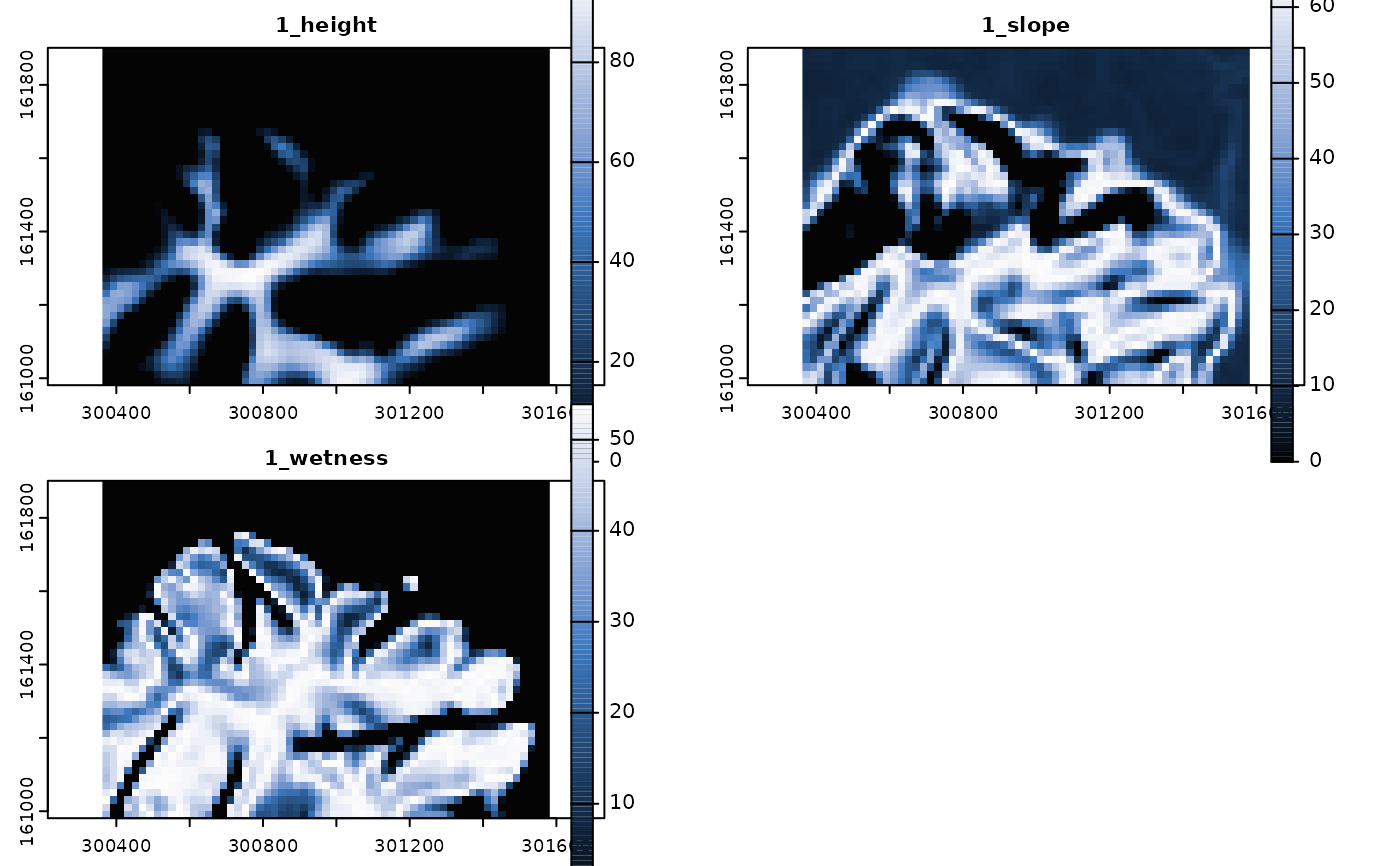
# Plot predicted distribution functions
if(interactive()){plot(tpdif, col = hcl.colors(100, "Oslo", rev = TRUE))}


#--------
# Writing results to disk and parallel processing

if(interactive()){
  # Directory for temporary files
  o <- tempdir()
  # Register parallel backend
  require(doParallel)
  registerDoParallel(4)
  # Predict distribution functions
  tpdif <- predict_functions(cuvar.rast = tcuvars,
                             cu.ind = 1,
                             cu = tdif$Class.Unit[1:3],
                             vars = tdif$Variable[1:3],
                             dif = tdif$Dist.Func[1:3],
                             grid.mult = 3, span = 0.9,
                             to.disk = TRUE,
                             outdir = o
                         )
   # Stop cluster
   stopImplicitCluster()
   # Clean temporary files
   file.remove(sources(tpdif))
 }
#> [1] TRUE TRUE TRUE